Plot a spectral track as a spectrogram

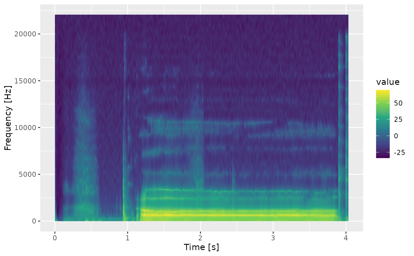
A ggplot2 layer that draws a multi-column spectral track of an AsspDataObj as a time x frequency raster, with the track values (dB for the package's spectra) on the fill scale.

Usage

geom_spectrogram(
  mapping = NULL,
  data = NULL,
  ...,
  tracks = NULL,
  time = "frame_time",
  freq_hz_per_bin = NULL,
  na.zeros = FALSE,
  na.rm = FALSE,
  interpolate = FALSE,
  show.legend = NA,
  inherit.aes = FALSE
)

Arguments

mapping

Set of aesthetic mappings created by ggplot2::aes(), applied to the time x frequency table the layer prepares (frame_time, freq, value). When NULL (default) the spectrum is drawn with aes(x = frame_time, y = freq, fill = value).

data

The data to display: an AsspDataObj holding a spectrum (from trk_dft_spectrum(), trk_lps_spectrum(), trk_css_spectrum() or any other multi-column track), the wide table from as.data.frame.AsspDataObj(), or an already long table. Inherited from the plot when NULL.

...

Other arguments passed on to ggplot2::layer().

tracks

Character. The spectral track to draw when data holds more than one multi-column track. NULL (default) uses the only one.

time

Character. Preferred name of the time column of data. The plotted table always names it frame_time.

freq_hz_per_bin

Numeric. Spacing between the coefficients in Hz, overriding the spacing derived from the origFreq of the object. Needed when data carries no sample rate.

na.zeros

Logical. Convert stored zeros to NA, leaving those raster cells unfilled. Default: FALSE.

na.rm

Logical. Remove NA values before drawing. Default: FALSE.

interpolate

Logical. Interpolate the raster for a smoother image. Default: FALSE.

show.legend, inherit.aes

Passed on to ggplot2::layer(), with ggplot2's usual defaults except inherit.aes = FALSE (see Details).

Value

A ggplot2 layer.

Details

SSFF stores a spectrum from 0 Hz up to the Nyquist rate, so the coefficients of a track with n columns sit at 0, bin_hz, ..., (n - 1) * bin_hz with bin_hz = origFreq / (2 * (n - 1)): a 2048-point spectrum of 44.1 kHz audio has 1025 bins of ~21.5 Hz. The track must be a frequency-domain track and data must hold exactly one multi-column track, or tracks must pick it; multi-column tracks of anything else (formants, LPC coefficients) belong to geom_track(). The raster is drawn by ggplot2::geom_raster()'s engine, which needs evenly spaced times and frequencies (all spectra in this package are evenly spaced). Zoom with ggplot2::coord_cartesian() rather than scale limits to keep the raster intact.

See also

geom_track() for single-value tracks and waveforms, ggtrack() for automatic track labels.

Examples

wav <- system.file("samples", "sustained", "a1.wav", package = "superassp")
# \donttest{
if (requireNamespace("ggplot2", quietly = TRUE)) {
  library(ggplot2)

  dft <- trk_dft_spectrum(wav, toFile = FALSE, verbose = FALSE)
  ggplot() +
    geom_spectrogram(data = dft) +
    coord_cartesian(ylim = c(0, 5000))

  # an object inherited from the plot works the same way
  lps <- trk_lps_spectrum(wav, toFile = FALSE, verbose = FALSE)
  ggtrack(lps) +
    geom_spectrogram() +
    labs(y = "Frequency [Hz]") +
    scale_fill_viridis_c()
}

# }