Create ggplot with automatic track labels

Creates a ggplot2 plot with automatic axis labels derived from track names. This is a convenience wrapper around ggplot() that automatically extracts and applies appropriate labels for acoustic track data.

Usage

ggtrack(
  data,
  mapping = ggplot2::aes(),
  ...,
  full_labels = FALSE,
  use_subscripts = TRUE
)

Arguments

data

data.frame, tibble, AsspDataObj or JsonTrackObj. Track data, either as a table from as.data.frame.AsspDataObj() or as the object itself.

mapping

ggplot2::aes() specification. Aesthetic mappings.

...

Additional ggplot2 layers to add (geoms, scales, themes, etc.).

full_labels

Logical. If TRUE, use full descriptive labels. If FALSE (default), use short labels suitable for plot axes.

use_subscripts

Logical. If TRUE (default), use plotmath expressions with subscripts (fo and F1 rendered with subscript digits). If FALSE, use plain text.

Value

A ggplot object with automatic axis labels.

Details

This function simplifies plotting of acoustic track data by automatically generating appropriate axis labels based on column names. It extracts the x and y variables from the aesthetic mapping and applies labels using get_track_label(). When no mapping is given, the axes are labelled for the layers this package provides: x becomes "Time [s]" for a table with a frame_time column, and y becomes the track label when the data holds exactly one track (ggtrack(rms) + geom_track()). Short labels (full_labels = FALSE, default):

• "fo [Hz]", "F1 [Hz]", "H1-H2c [dB]"

• Concise, suitable for most plots Full labels (full_labels = TRUE):

• "Frequency of oscillation [Hz]"

• "First formant frequency [Hz]"

• "H1-H2 corrected for formants [dB]"

• Descriptive, suitable for publications Additional layers can be added using the ... argument or by adding to the returned ggplot object with +.

See also

• geom_track() and geom_spectrogram() for the layers to combine with

• as.data.frame.AsspDataObj() for the wide track table

• get_track_label() for label extraction

• ggplot2::ggplot() for the underlying plotting function

Examples

wav <- system.file("samples", "sustained", "a1.wav", package = "superassp")
# \donttest{
if (requireNamespace("ggplot2", quietly = TRUE)) {
  library(ggplot2)

  # tracks of the object, labels taken from the track metadata
  f0 <- trk_pitch_ksv(wav, toFile = FALSE, verbose = FALSE)
  ggtrack(f0) + geom_track()

  # y-axis: "fo [Hz]"
  # a spectrogram of a spectrum track
  dft <- trk_dft_spectrum(wav, toFile = FALSE, verbose = FALSE)
  ggtrack(dft) + geom_spectrogram() + labs(y = "Frequency [Hz]")

  # the wide table with a column-wise mapping. convert_units = FALSE keeps
  # the columns plain numeric; unit-assigned columns are "units" objects,
  # which ggplot2 can only scale with the units package attached.
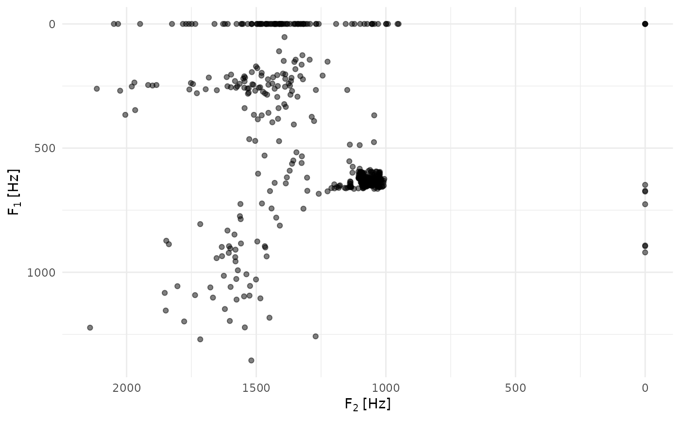
  fms <- trk_formant_forest(wav, numFormants = 3, toFile = FALSE, verbose = FALSE)
  df_fms <- as.data.frame(fms, convert_units = FALSE)
  ggtrack(df_fms, aes(x = F2_Hz, y = F1_Hz)) +
    geom_point(alpha = 0.5) +
    scale_x_reverse() +
    scale_y_reverse() +
    theme_minimal()
  # Automatic labels: "F1 [Hz]", "F2 [Hz]"
}

# }