Plot time-aligned tracks of an AsspDataObj

A ggplot2 layer that draws the tracks of an AsspDataObj (or of the wide table written by as.data.frame.AsspDataObj()) as one line per track, against time in seconds. Scales, facets, coordinates, legends and themes apply as with any other layer.

Usage

geom_track(
  mapping = NULL,
  data = NULL,
  ...,
  tracks = NULL,
  time = "frame_time",
  na.zeros = FALSE,
  na.rm = FALSE,
  show.legend = NA,
  inherit.aes = FALSE,
  stat = "identity",
  position = "identity"
)

Arguments

mapping

Set of aesthetic mappings created by ggplot2::aes(), applied to the track table the layer prepares (frame_time, value, track, band, bin). When NULL (default) the tracks are drawn with aes(x = frame_time, y = value, colour = track, group = track).

data

The data to display: an AsspDataObj (from a trk_* function, read_audio(), read_ssff() or read_track()), the wide table from as.data.frame.AsspDataObj(), or an already long track table with frame_time, value and track columns. Inherited from the plot when NULL.

...

Other arguments passed on to ggplot2::layer().

tracks

Character. Tracks to plot, matched against the column name ("RMS_dB"), the track template ("RMS[dB]") or the object's track name. NULL (default) plots every track.

time

Character. Preferred name of the time column of data. The plotted table always names it frame_time.

na.zeros

Logical. Convert stored zeros to NA, so that undefined frames (unvoiced f0, absent formants) break the line instead of dropping to zero. Default: FALSE.

na.rm

Logical. Remove NA values before drawing. Default: FALSE.

show.legend, inherit.aes, stat, position

Passed on to ggplot2::layer(), with ggplot2's usual defaults except inherit.aes = FALSE (see Details).

Value

A ggplot2 layer.

Details

Track data is rewritten into a long table (frame_time, value, track, band, bin) before the layer is built, because ggplot2 hands a layer only its evaluated aesthetics. A mapping therefore refers to that table, and inherit.aes defaults to FALSE: the mapping goes on the layer, as in geom_track(data = obj, mapping = aes(x = frame_time, y = value, group = track)). tracks also matches bands, so tracks = "Fi[Hz]" draws F1..Fn while tracks = "F1_Hz" draws a single formant. For a column-wise plot of the wide table (one column against another), use ggplot2::geom_line() or ggplot2::geom_point() on as.data.frame.AsspDataObj() instead: ggtrack(df, aes(x = F2_Hz, y = F1_Hz)) + geom_point(). 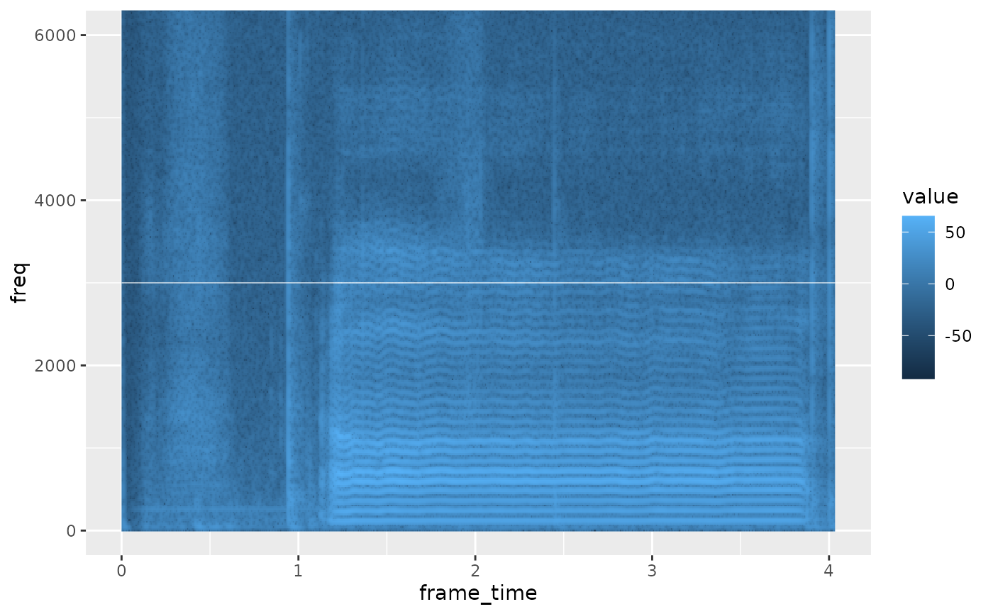Layers on different objects compose, so a waveform can be drawn over a spectrogram by adding one geom_spectrogram() and one geom_track(). The layer carries one row per record and track (a waveform has one row per sample), so window a long recording at read time with read_audio(wav, begin = …, end = …).

See also

geom_spectrogram() for multi-column spectral tracks, ggtrack() for automatic track labels, as.data.frame.AsspDataObj() for the wide table.

Examples

wav <- system.file("samples", "sustained", "a1.wav", package = "superassp")
# \donttest{
if (requireNamespace("ggplot2", quietly = TRUE)) {
  library(ggplot2)

  # every track of the object, one line each
  rms <- trk_rms(wav, toFile = FALSE, verbose = FALSE)
  ggplot() + geom_track(data = rms)

  # a subset, labelled from the track metadata
  fms <- trk_formant_forest(wav, numFormants = 3, toFile = FALSE, verbose = FALSE)
  ggtrack(fms) + geom_track(tracks = c("F1_Hz", "F2_Hz", "F3_Hz"))

  # the raw waveform
  audio <- read_audio(wav, samples = TRUE)
  ggplot() + geom_track(data = audio)

  # a waveform drawn over the spectrogram of the same file
  dft <- trk_dft_spectrum(wav, toFile = FALSE, verbose = FALSE)
  ggplot() +
    geom_spectrogram(data = dft) +
    geom_track(data = audio,
               mapping = aes(x = frame_time, y = value / 8000 + 3000),
               colour = "white", linewidth = 0.2) +
    coord_cartesian(ylim = c(0, 6000))
}

# }