Auditory Modeling with Cochleagram and Excitation

Introduction

pladdrr provides auditory modeling through the Cochleagram and Excitation objects. These model how the human auditory system processes acoustic information, as opposed to a purely physical (

spectral) analysis.

Key Concepts

Cochleagram: Models the basilar membrane response in the cochlea using the Bark scale (

0-25.6 Bark ≈ 0-20,000 Hz)
Excitation: Represents auditory nerve firing patterns on the ERB ( Equivalent Rectangular Bandwidth) scale
Loudness: Perceptual loudness measured in sones (not physical intensity)
Perceptual Distance: Quantifies how different two sounds “sound” to human listeners

library(pladdrr)
#> pladdrr: direct access to Praat's core algorithms from R.
#> See ?pladdrr for an overview, or citation("pladdrr") for citation details.
library(ggplot2)

Cochleagram Analysis

Creating a Cochleagram

The cochleagram represents sound on a frequency scale that matches the human cochlea’s tonotopic organization.

# Load or create a sound
sound <- Sound$create_tone(frequency = 440, duration = 0.5,
  sampling_rate = 44100)

# Create cochleagram
cochlea <- sound$to_cochleagram(
  dt = 0.01,                    # Time step (10 ms)
  df = 0.1,                     # Frequency step in Bark
  window_length = 0.025,        # Analysis window (25 ms)
  forward_masking_time = 0.03   # Temporal masking (30 ms)
)

Understanding the Bark Scale

The Bark scale is a perceptual frequency scale where: - 1 Bark ≈ 1 critical band (frequency resolution of human hearing) - 0 Bark = 0 Hz - 13 Bark ≈ 1500 Hz (center of speech range) - 25.6 Bark ≈ 20,000 Hz

# Common frequency conversions
# F1 (250 Hz) ≈ 2.5 Bark
# F2 (2000 Hz) ≈ 15 Bark
# F3 (3000 Hz) ≈ 19 Bark

Querying Cochleagram Values

# Get excitation at specific time and frequency
# 440 Hz ≈ 4.2 Bark
excitation_440hz <- cochlea$get_value_at_time_and_frequency(
  time = 0.25,      # At 250 ms
  freq_bark = 4.2   # ~440 Hz
)

print(paste("Excitation at 440 Hz:", round(excitation_440hz, 4)))
#> [1] "Excitation at 440 Hz: 79.7166"

Visualizing Cochleagrams

# Export to matrix for plotting
cochlea_matrix <- as.matrix(cochlea$as_matrix())

# Convert to long format for ggplot2 (rows = frequency bands, columns = time
#  frames)
times <- vapply(seq_len(cochlea$get_number_of_frames()),
  cochlea$get_time_from_column, numeric(1))
barks <- vapply(seq_len(cochlea$get_number_of_frequency_bands()),
  cochlea$get_frequency_from_row, numeric(1))
df_long <- expand.grid(Bark = barks, Time = times)
df_long$Excitation <- as.vector(cochlea_matrix)

# Plot
ggplot(df_long, aes(x = Time, y = Bark, fill = Excitation)) +
  geom_raster() +
  scale_fill_viridis_c(option = "inferno") +
  labs(
    title = "Cochleagram of 440 Hz Tone",
    x = "Time (s)",
    y = "Frequency (Bark)",
    fill = "Excitation"
  ) +
  theme_minimal()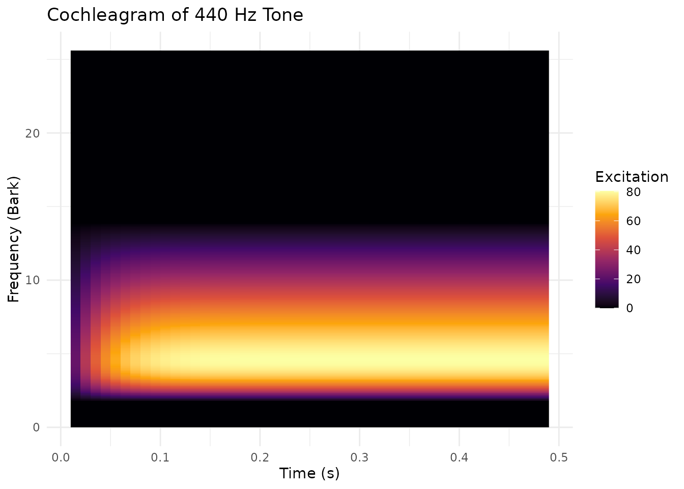

Advanced: Ear-Drum-Brain Model

For more realistic auditory modeling, use the EDB ( Ear-Drum-Brain) method which includes synaptic processing:

cochlea_edb <- sound$to_cochleagram_edb(
  dtime = 0.01,
  dfreq = 0.1,
  has_synapse = TRUE,         # Include synaptic adaptation
  replenishment_rate = 0.01,  # Neurotransmitter replenishment
  loss_rate = 0.1,            # Synaptic depletion
  return_rate = 0.05,         # Recovery rate
  reprocessing_rate = 0.01    # Reprocessing rate
)

The EDB model is more computationally intensive but provides: - Synaptic adaptation (important for continuous sounds) - More realistic temporal response - Better modeling of masking effects

Excitation Patterns

Creating Excitation from Spectrum

Excitation patterns represent the instantaneous firing rate of auditory nerve fibers:

# Create excitation from spectrum
spectrum <- sound$to_spectrum()
excitation <- spectrum$to_excitation(erb_density = 0.1)

# Get perceptual loudness
loudness <- excitation$get_loudness()
print(paste("Loudness:", round(loudness, 2), "sones"))
#> [1] "Loudness: 106.49 sones"

Creating Excitation from Cochleagram

You can also extract excitation patterns at specific times from a cochleagram:

# Extract excitation pattern at t = 0.25s
excitation_t <- cochlea$to_excitation(0.25)

# Query excitation at specific frequency
exc_value <- excitation_t$get_value_at_frequency(4.2)  # ~440 Hz
print(paste("Excitation at 440 Hz:", round(exc_value, 4)))
#> [1] "Excitation at 440 Hz: 79.7166"

Perceptual Distance

Quantify how different two sounds are perceptually:

# Create two different sounds
sound1 <- Sound$create_tone(frequency = 440, duration = 0.2,
  sampling_rate = 22050)
sound2 <- Sound$create_tone(frequency = 550, duration = 0.2,
  sampling_rate = 22050)

# Get excitation patterns
exc1 <- sound1$to_spectrum()$to_excitation()
exc2 <- sound2$to_spectrum()$to_excitation()

# Calculate perceptual distance
distance <- exc1$get_distance(exc2)
print(paste("Perceptual distance:", round(distance, 4)))
#> [1] "Perceptual distance: 6.3688"

Higher distance values indicate sounds that are more perceptually different.

Clinical Applications

Hearing Loss Simulation

Compare cochleagrams of normal and impaired hearing:

# Original speech sound
sound_original <- Sound$new(
  system.file("extdata", "test.wav", package = "pladdrr"))

# In practice, apply a low-pass filter to sound_filtered here to simulate
# high-frequency hearing loss (Sound objects have no clone() method, so
# start from a fresh load rather than copying sound_original)
sound_filtered <- Sound$new(
  system.file("extdata", "test.wav", package = "pladdrr"))

# Create cochleagrams
cochlea_normal <- sound_original$to_cochleagram()
cochlea_impaired <- sound_filtered$to_cochleagram()

# Calculate perceptual difference
difference <- cochlea_normal$get_difference(
  cochlea_impaired,
  tmin = 0,
  tmax = 0  # Full duration
)

print(paste("Hearing loss impact (distance):", round(difference, 4)))
#> [1] "Hearing loss impact (distance): 0"

Without an actual filtering step, sound_original and sound_filtered are identical here, so difference is 0; apply a real low-pass filter to sound_filtered to get a non-zero result.

Speech Intelligibility Prediction

Excitation patterns can predict speech intelligibility. This requires two recordings of the same material (clean and noisy); the pattern below uses the bundled test file for both, so distance will be 0.

# Clean speech
speech_clean <- Sound$new(
  system.file("extdata", "test.wav", package = "pladdrr"))

# Noisy speech (in practice, a separate recording made in noise)
speech_noisy <- Sound$new(
  system.file("extdata", "test.wav", package = "pladdrr"))

# Get excitation patterns
exc_clean <- speech_clean$to_spectrum()$to_excitation()
exc_noisy <- speech_noisy$to_spectrum()$to_excitation()

# Perceptual distance correlates with intelligibility loss
distance <- exc_clean$get_distance(exc_noisy)

# Lower distance = better preserved intelligibility
distance
#> [1] 0

Loudness Recruitment Assessment

Track loudness perception across intensity levels:

# Create sounds at different relative levels by scaling tone amplitude
intensities <- seq(40, 80, by = 10)  # relative dB SPL
loudnesses <- numeric(length(intensities))

for (i in seq_along(intensities)) {
  # Approximate a level in dB by scaling amplitude (20*log10(amplitude))
  amplitude <- min(0.99, 10 ^ ((intensities[i] - 80) / 20))
  sound <- Sound$create_tone(frequency = 1000, duration = 0.3,
                             amplitude = amplitude, sampling_rate = 44100)

  # Measure perceptual loudness
  excitation <- sound$to_spectrum()$to_excitation()
  loudnesses[i] <- excitation$get_loudness()
}

# Plot loudness growth function
plot(intensities, loudnesses,
     xlab = "Intensity (dB SPL)",
     ylab = "Loudness (sones)",
     main = "Loudness Growth Function",
     type = "b")

Formant Extraction from Excitation

Excitation patterns provide an alternative method for formant extraction:

# Create vowel sound
sound_vowel <- Sound$create_tone(duration = 0.2, sampling_rate = 22050)

# Get excitation pattern
excitation <- sound_vowel$to_spectrum()$to_excitation()

# Extract formants from excitation pattern
formant <- excitation$to_formant(max_formants = 5)

# Query formants
f1 <- formant$get_value_at_time(1, 0.1, unit = "hertz")
f2 <- formant$get_value_at_time(2, 0.1, unit = "hertz")

if (!is.na(f1) && !is.na(f2)) {
  print(paste("F1:", round(f1), "Hz"))
  print(paste("F2:", round(f2), "Hz"))
}

This method can be more robust than LPC for: - Noisy speech - Breathy voice quality - Non-modal phonation

Best Practices

Choosing Parameters

Cochleagram time step (dt): - Speech analysis: 0.005-0.010 s (5-10 ms) - Music: 0.010-0.020 s - Sustained sounds: 0.020-0.050 s

Frequency step (df): - Detailed analysis: 0.05-0.1 Bark - Standard analysis: 0.1-0.2 Bark - Coarse analysis: 0.2-0.5 Bark

Window length: - Shorter (0.005-0.010 s): Better time resolution - Medium (0.020-0.030 s): Balanced - Longer (0.050-0.100 s): Better frequency resolution

Forward masking: - Standard: 0.03 s - Strong masking: 0.05-0.1 s - Minimal masking: 0.01-0.02 s

Performance Considerations

# For batch processing, reuse objects when possible
sounds <- list(sound1, sound2, sound_vowel)

# Vectorized approach: build the cochleagrams once, then query all of them
cochleagrams <- lapply(sounds, function(s) {
  s$to_cochleagram(dt = 0.01, df = 0.1)
})

# Extract loudness from all
loudnesses <- vapply(cochleagrams, function(c) {
  c$get_loudness_at_time(0.1)
}, numeric(1))

Memory Management

Cochleagrams and excitation patterns can be large. Clean up when done:

# Process and extract only what you need
cochlea <- sound$to_cochleagram()
loudness_time_series <- vapply(seq(0, 0.5, by = 0.01),
  cochlea$get_loudness_at_time, numeric(1))

# Remove large object if no longer needed
rm(cochlea)
gc()  # Force garbage collection
#>           used  (Mb) gc trigger (Mb) max used  (Mb)
#> Ncells 1889262 100.9    3182971  170  3182971 170.0
#> Vcells 3212973  24.6    8388608   64  7264761  55.5

Comparison with Traditional Analysis

Traditional	Auditory Modeling
Spectrogram (linear/log Hz)	Cochleagram (Bark scale)
Spectrum power (dB)	Excitation (nerve firing rate)
Sound level (dB SPL)	Loudness (sones)
Spectral distance (Euclidean)	Perceptual distance

Auditory modeling is preferred when: - Modeling human perception - Clinical audiology applications - Speech intelligibility prediction - Psychoacoustic research - Hearing aid algorithm development

Session Info

sessionInfo()
#> R version 4.6.1 (2026-06-24)
#> Platform: x86_64-pc-linux-gnu
#> Running under: Ubuntu 24.04.5 LTS
#> 
#> Matrix products: default
#> BLAS:   /usr/lib/x86_64-linux-gnu/openblas-pthread/libblas.so.3 
#> LAPACK: /usr/lib/x86_64-linux-gnu/openblas-pthread/libopenblasp-r0.3.26.so;  LAPACK version 3.12.0
#> 
#> locale:
#>  [1] LC_CTYPE=C.UTF-8       LC_NUMERIC=C           LC_TIME=C.UTF-8       
#>  [4] LC_COLLATE=C.UTF-8     LC_MONETARY=C.UTF-8    LC_MESSAGES=C.UTF-8   
#>  [7] LC_PAPER=C.UTF-8       LC_NAME=C              LC_ADDRESS=C          
#> [10] LC_TELEPHONE=C         LC_MEASUREMENT=C.UTF-8 LC_IDENTIFICATION=C   
#> 
#> time zone: UTC
#> tzcode source: system (glibc)
#> 
#> attached base packages:
#> [1] stats     graphics  grDevices utils     datasets  methods   base     
#> 
#> other attached packages:
#> [1] ggplot2_4.0.3 pladdrr_5.0.5
#> 
#> loaded via a namespace (and not attached):
#>  [1] gtable_0.3.6        jsonlite_2.0.0      dplyr_1.2.1        
#>  [4] compiler_4.6.1      tidyselect_1.2.1    Rcpp_1.1.2         
#>  [7] jquerylib_0.1.4     systemfonts_1.3.2   scales_1.4.0       
#> [10] textshaping_1.0.5   yaml_2.3.12         fastmap_1.2.0      
#> [13] R6_2.6.1            labeling_0.4.3      generics_0.1.4     
#> [16] knitr_1.52          tibble_3.3.1        desc_1.4.3         
#> [19] bslib_0.12.0        pillar_1.11.1       RColorBrewer_1.1-3 
#> [22] rlang_1.3.0         cachem_1.1.0        xfun_0.60          
#> [25] fs_2.1.0            sass_0.4.10         S7_0.2.2           
#> [28] otel_0.2.0          viridisLite_0.4.3   cli_3.6.6          
#> [31] pkgdown_2.2.1       withr_3.0.3         magrittr_2.0.5     
#> [34] digest_0.6.39       grid_4.6.1          lifecycle_1.0.5    
#> [37] vctrs_0.7.3         evaluate_1.0.5      glue_1.8.1         
#> [40] data.table_1.18.6.1 farver_2.1.2        codetools_0.2-20   
#> [43] ragg_1.5.2          rmarkdown_2.32      tools_4.6.1        
#> [46] pkgconfig_2.0.3     htmltools_0.5.9